Confusion Matrix

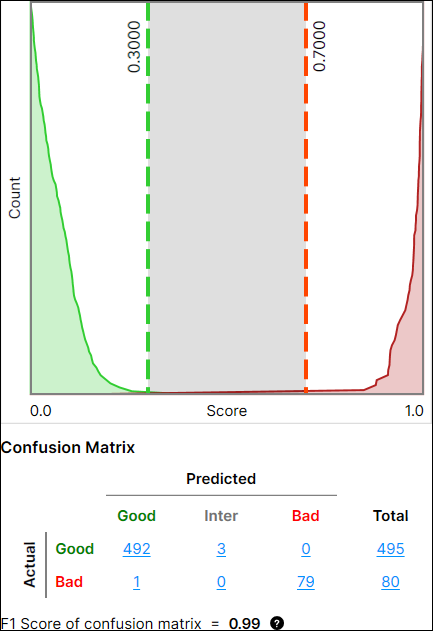
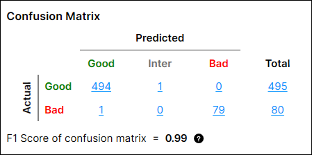
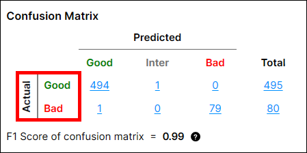
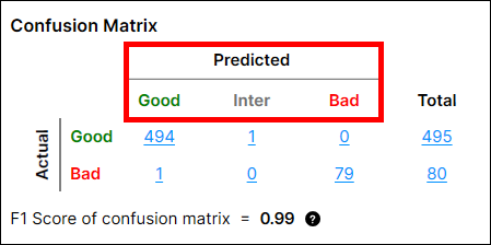
The Confusion Matrix is a visual representation of the ground truth versus the tool's predictions. The confusion matrix in Red Analyze Tool is a comparison table of the tool processing results showing the relationships between the Actual values and the Predicted values. The confusion matrix and its performance metrics (the precision, recall, and F1 score of confusion matrix), which will be explained more below, are offered both in Red Analyze Supervised (Red Analyze Focused Supervised, Red Analyze High Detail) and Red Analyze Focused Unsupervised.

Counting Confusion Matrix

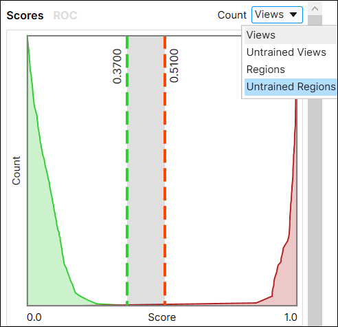
There are 4 ways to populate this table by Count dropdown option: Views, Untrained Views, Regions, and Untrained region. These are also used to draw "Score" graph (Score Distribution Graph).

Views: A label and a marking are imprinted on each view
Untrained Views: A label and a marking are imprinted on each view that does not belong to the training set.
Regions: A label and a marking are imprinted on each region in a view. Regions are split into the defect regions (bad) and the backgrounds (good), labeled and marked as per them.
Untrained Regions: A label and a marking are imprinted on each pixel in a view that does not belong to the training set. Regions are split into the defects (bad pixels) and the background (good pixels), labeled and marked as per them.

Note:
There are two types of labeling for Red Analyze: Pixel-wise labeling and view-wise labeling.

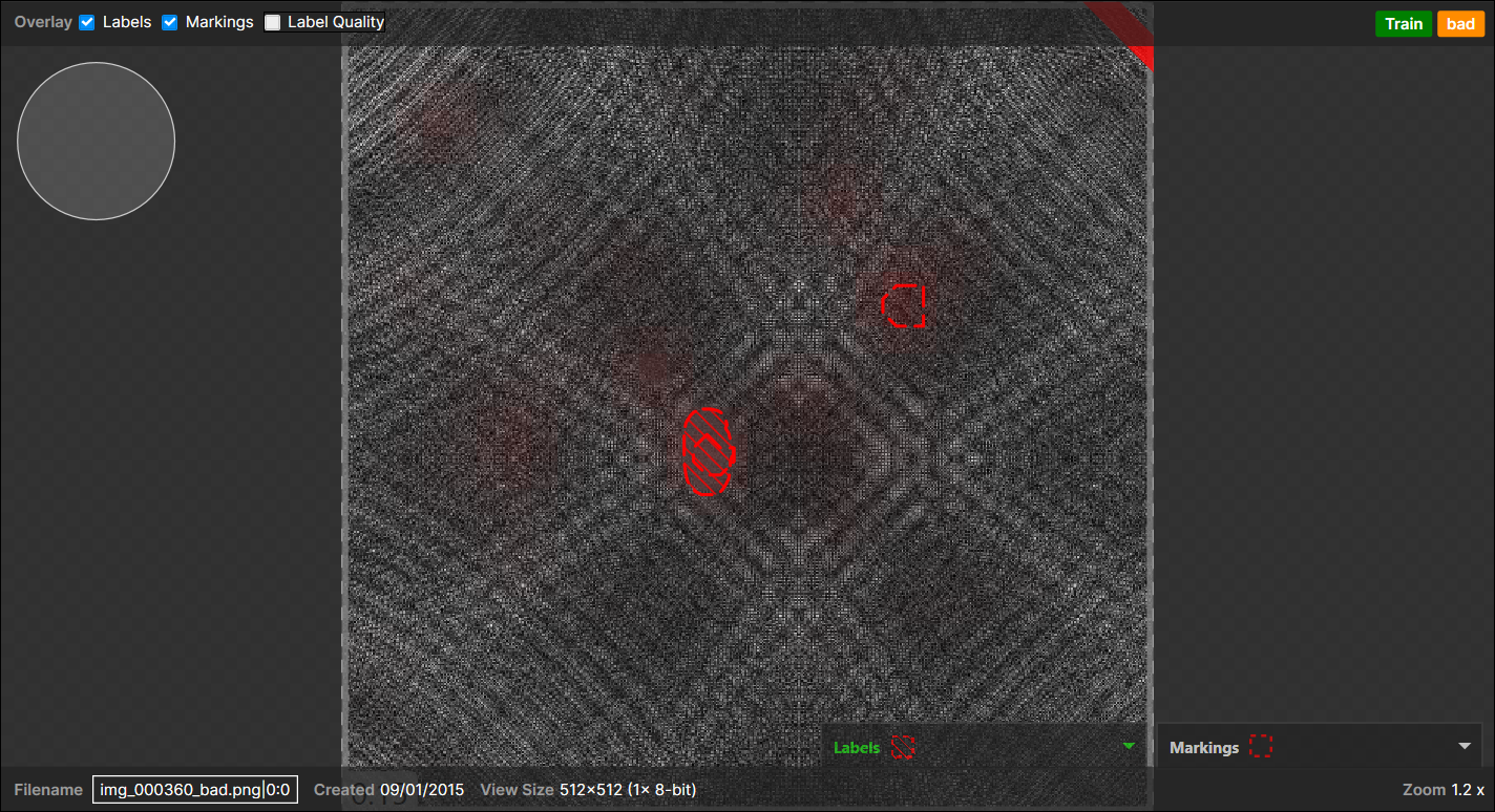
Pixel-wise labeling: right-click on Image Display Area → click "Edit Regions" → draw a defect region and click "Apply"
View-wise labeling: right-click on a view in View Browser→ click "Label Views" → select "Bad"

When you label an entire view itself as "Bad"(view-wise), and that is view-wise labeling used in Views/Untrained Views. But when you label one or more pixels as "Bad" (pixel-wise), and that is pixel-wise labeling used in Regions/Untrained Regions.

For Regions/Untrained Regions, a pixel that is not labeled at all is considered to be labeled as "Good" (The backgrounds). The marking is the prediction of whether a pixel is a defect pixel or not by checking the defect probability of this pixel goes over T1. Note that a view that has pixel-wise defect label(s) is automatically also labeled as "Bad" in view level.

Confusion Matrix Calculation - Views/Untrained Views

In Red Analyze tools, the confusion matrix can be calculated based on a region or a view. The values of confusion matrix are clearly different from which basis is selected.

When it is view-basis, the marking is made on each view, not each region. For a view, if there are defect pixels in this view whose score(s) are good enough to go over T2 threshold, then it is predicted as "Bad," otherwise, good or inter.

To mark a view as "Bad," the defect pixel with the highest defect probability (score) could be anywhere in a view, which doesn't necessarily be in the labeled defect region.

When it is view-basis, the label is made on each view, not each region. If you label a view as "Bad," that is said and it is labeled as bad, and otherwise, "Good."

How to calculate "Actuals" - Views/Untrained Views

When a view with "Good" label is given,
→ 1 "Good" Actual.
When a view with "Bad" label is given,
→ 1 "Bad" Actual.

How to calculate "Predicted" - Views/Untrained Views

When it is view-basis, the prediction is made on each "Actual" view, which is found above, not on each region. The prediction is calculated from T1, T2 and the representative score of the actual view.

The representative score of a view is the highest score of pixels in this view. Each score is the defect probability of each pixel. For example, for a view, if there are defect pixels in this view whose score(s) are good enough to go over T2 threshold, then it is predicted as "Bad," otherwise, "Good or Inter."

When the highest score from all pixels in a view < T1,
→ 1 "Good" Predicted.
When the highest score from all pixels in a view > T2,
→ 1 "Bad" Predicted.
Otherwise,
→ 1 "Inter" Predicted.

Tip: Summary of Counting "Actuals" - Views/Untrained Views
1 "Good" labeled view → 1 actual "Good" view,
1 "Bad" labeled view → 1 actual "Bad" view

Tip: Summary of Counting "Predicts" - Views/Untrained Views
The highest score from all pixels in a view < T1 → 1 predicted "Good" view,
The highest score from all pixels in a view > T2 → 1 predicted "Bad" view,
Otherwise, 1 predicted "Inter" view

Confusion Matrix Calculation - Regions/Untrained Regions

In Red Analyze tools, the confusion matrix can be calculated on the basis of region or views. The values of confusion matrix are clearly different from which basis is selected.

When it is region-basis, the labeling and marking are made on each region, not each view. This means that multiple marked regions (a 'marked region' stands for a set of pixels that are marked as "defective" with respect to T1 and T2) in a view are included in the confusion matrix calculation. In other words, a single view could be used to produce multiple counts (actual - predicted pairs) in the confusion matrix table, whereas a single view only produces a single count in the table in Views/Untrained Views.

How to calculate "Actuals" - Regions/Untrained Regions

Compared to Views/Untrained Views, when it comes to counting "actual" for the confusion matrix for regions/untrained regions, there is a different logic for counting "actual."

When a view with "Good" label is given,
→ 1 "Good" Actual region
(The entire view itself is considered as a background region).

When a view with "Bad" label and with N pixel-wise labeled defect regions is given,
→ N "Bad" Actuals corresponding to the number of pixel-wise labeled regions in this view (N "Bad" actual regions).
→ 1 "Good" Actual region corresponding to all the background pixels in this view.

When a view with "Bad" label and without pixel-wise labeled defect regions is given,
→ 1 "Bad" Actual.

How to calculate "Predicted" - Regions/Untrained Regions

In the confusion matrix for regions or untrained regions, the prediction is made on each "Actual" region, whose calculation was illustrated in the section right above. The prediction is calculated from T1, T2 and the representative score of an actual region.

The representative score of the actual region is the highest score of pixels in the "actual" region area. This is just the same as that the representative score of a view is the highest score of pixels in that view. Each score is the defect probability of each pixel.

In the confusion matrix for regions or untrained regions, the predicted result is determined by T1, T2 and the score of the actual region:

The score of actual region < T1,
→ 1 "Good" Predicted

T1 < The score of actual region < T2,
→ 1 "Inter" Predicted

The score of actual region > T2,
→ 1 "Bad" Predicted

Examples of Actual-Predicted pair calculation for Regions/Untrained Regions

To make the examples below more clear, here we assume that the highest score found from an actual region is higher than T2.

When N marked regions appear on the backgrounds (the good labeled pixels) and there are no pixel-wised labeled defects and this view itself was labeled as "Good":
→ 1 (Actual) Good - (Predicted) Bad pair
(N marked regions are considered as a single marked region)

Example of 3 marked regions appear on the backgrounds, no pixel-wise labeled defects, "Good" labeled view:
When N marked regions appear on the backgrounds (the good labeled pixels) and there are no pixel-wised labeled defects but this whole view itself was just labeled as "Bad":
→ 1 (Actual) Bad - (Predicted) Bad pair
(N marked regions are considered as a single marked region)

Example of 4 marked regions appear on the backgrounds, no pixel-wise labeled defects, "Bad" labeled view:
When marked regions appear on the pixel-wise labeled defect regions:
The one important thing here to decide the outcome is, of the total, how many marked regions are overlapped with the pixel-wise labeled defect regions:
- <Case 1>
  
  1 pixel-wise labeled region,
  1 marked region (overlapped with the pixel-wise labeled region),
  1 marked region (not overlapped with the pixel-wise labeled region and appear on the background):
  →
  1 (Actual) Bad - (Predicted) Bad pair (overlapped),
  1 (Actual) Good - (Predicted) Bad pair (not overlapped),
  
  Note: When there are one or more pixel-wise labeled defect regions in a view, all the pixels all of a lump except the labeled regions are considered as "a background," which counts for 1 Actual "Good" region." This expands to most cases but does not apply when there are no pixel-wise labeled regions in the view but the view itself was labeled as "Bad."
  
  Example of a marked region appear on the backgrounds, another marked region appear on a pixel-wise labeled region (overlapped), and this view itself is labeled as "Bad" as there are one or more pixel-wise labeled defects:
- <Case 2>
  
  5 pixel-wise labeled regions,
  3 marked regions (each overlapped with each pixel-wise labeled region),
  2 marked regions (not overlapped with any pixel-wise labeled region and appear on the background):
  →
  3 (Actual) Bad - (Predicted) Bad pair (overlapped),
  2 (Actual) Bad - (Predicted) Good pair (not overlapped),
  1 (Actual) Good - (Predicted) Bad pair
  
  Note: The 2 marked regions appeared in the background are considered as a single marked region, which results in 1 "Bad" Predicted. This also expands to the N marked regions case.
- <Case 3>
  
  3 pixel-wise labeled regions (A, B, C),
  3 marked regions (2 overlapped with A and 1 with B)
  1 marked region(not overlapped = appear on the background):
  →
  1 (Actual) Bad - (Predicted) Bad pair (2 overlapped with A),
  1 (Actual) Bad - (Predicted) Bad pair (1 overlapped with B),
  1 (Actual) Good - (Predicted) Bad pair (appear on the background),
  1 (Actual) Bad - (Predicted) Good pair (C)

Tip: Summary of Counting "Actuals" - Regions/Untrained Regions
1 "Good" labeled view → 1 actual "Good" region,
1 "Bad" labeled view without pixel-wise labeled region → 1 actual "Bad" region,
1 "Bad" labeled view with N pixel-wise labeled region,
→ 1 actual "Good" region + N actual Bad regions
(N is the number of defect regions that users drew)

Tip: Summary of Counting "Predicts" - Regions/Untrained Regions
The highest score from a labeled region < T1 → 1 predicted "Good" region,
The highest score from a labeled region > T2 → 1 predicted "Bad" region,
Otherwise, 1 predicted "Inter" region.

F1 Score Calculation

F1 Score of the confusion matrix is the combination of precision and recall, serving as a comprehensive metric for the segmentation performance. The recall represents how the neural network matches well the area of the labeled defect region and the precision represents how the neural network refrains well from being confused by other areas in an image. To get F1 Score of confusion matrix, the precision and recall must be calculated beforehand. Note that the precision, recall, and F1 score are calculated differently compared to those in Region Area Metrics, calculated in pixel level.

F1 Score of confusion matrix changes per the Count dropdown option. It is interpreted as the harmonic mean between the precision and recall of the current confusion matrix. If a view or a region is predicted as "Inter," it is counted as "Bad" for the calculation of precision, recall, and F1 Score.

(Actual Good , Predicted Inter) → (Actual Good, Predicted Bad)
(Actual Bad, Predicted Inter) → (Actual Bad, Predicted Bad)

Note: When the tool is in Supervised mode (High Detail and Focused Supervised), it contains the Region Area Metric, to denote data about the defect region.

Before introducing calculation methodology, here are the things that should be known for the calculation:

For predicting "Good" class:

1 "Actual Good - Predicted Good" pair stands for 1 "True Positive (TP)"
1 "Actual Bad - Predicted Good" pair stands for 1 "False Positive (FP)"
1 "Actual Bad - Predicted Bad" pair stands for 1 "True Negative (TN)"
1 "Actual Good - Predicted Bad" pair stands for 1 "False Negative (FN)"

For predicting "Bad" class:

1 "Actual Bad - Predicted Bad" pair stands for 1 "True Positive (TP)"
1 "Actual Good - Predicted Bad" pair stands for 1 "False Positive (FP)"
1 "Actual Good - Predicted Good" pair stands for 1 "True Negative (TN)"
1 "Actual Bad - Predicted Good" pair stands for 1 "False Negative (FN)"

From this setting, the calculation of the precision, recall, and F1 Score of confusion matrix for "Good" Class are done as below:

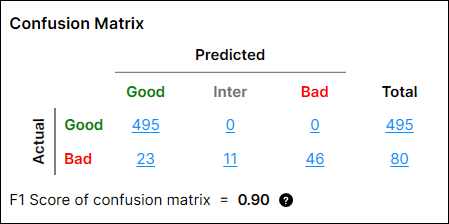
Precision = TP / (TP + FP) = 495/(495+23) = 0.956
Recall = TP / (TP + FN) = 495/(495+0) = 1
F-score = 2 * Recall * Precision / (Recall+Precision) = 2 * 0.956 * 1 / 1.956 = 0.978

The precision, recall, and F1 Score of confusion matrix for "Bad" Class is done as below:

Precision = TP/(TP+FP) = 57/(57+0) = 1
Recall = TP/(TP+FN) = 57/(57+23) = 0.713
F-score = 2 * Recall * Precision / (Recall + Precision) = 2 * 1 * 0.713 / 1.713= 0.832

Then, the F1 score of confusion matrix is:

0.5 * (F-score of Good class) + 0.5 * (F-score of Bad class) = 0.5 * 0.978 + 0.5 * 0.832 = 0.90


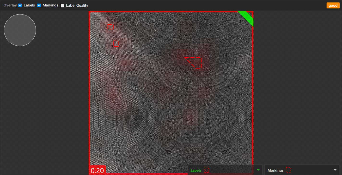
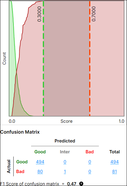
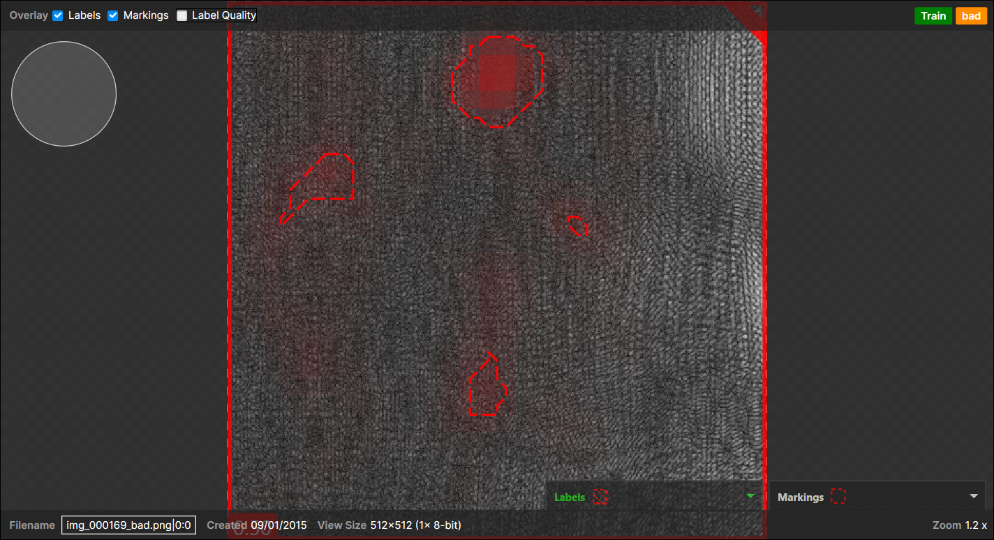
Good Performance	Poor Performance