VisionPro Deep Learning Tool Chains
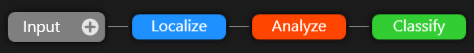
Each of the Cognex Deep Learning Tools has a unique output, and that output can be used an input to another tool, in what is referred to as tool chaining. In the image below, a Blue Locate Tool has a node model made up of the three features (H, B and T) which is providing a location (this is similar to using a pattern tool in a traditional vision application to create a fixture).
The location output by the Blue Locate tool is used by the Red Analyze Tool to orient and create its view, allowing the detection analysis to be performed in the same area of the image, based on the node model output by the Blue Locate tool. Finally, the Green Classify Tool is used to classify the output of the Red Analyze tool, based on the classification criteria established for the Green Classify tool.
Create a VisionPro Deep Learning Tool Chain
-
To create a chain of tools, after adding a tool, press the Add icon on the tool's icon.
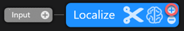
-
This way you can create a sequence of tools, where each tool is linked to the proceeding tool.
Define the ROI of a Downstream Tool
When tools are chained together, the tool before the next tool will determine the Region of Interest (ROI) toolbar options of the downstream tool.
ROI Options Following a Blue Locate Tool
When a Blue Locate Tool is the preceding tool, it can provide a transform that can be used by a downstream tool to fixture where the tool's region of interest will be located in the image.
These are the options to specify a region of interest for the downstream tool.
- One or more features
- A match
- A node model
- A layout model
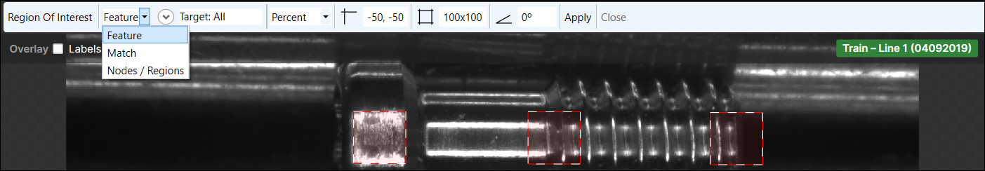
ROI from a Feature
You can also use the individual features defined in a Blue Locate tool to provide the region of interest for downstream tools. Each feature provides a five degree of freedom (DOF) transform (X translation, Y translation, rotation, X scale and Y scale).
The feature will also determine the size of the ROI. The percentage of the ROI will be based on the width and height of the feature.
-
Select Feature.
-
Press the down arrow beside the Target to reveal a drop-down menu that will contain a list of the features defined by the tool, and Matched Only, which will only return features that are part of a model.
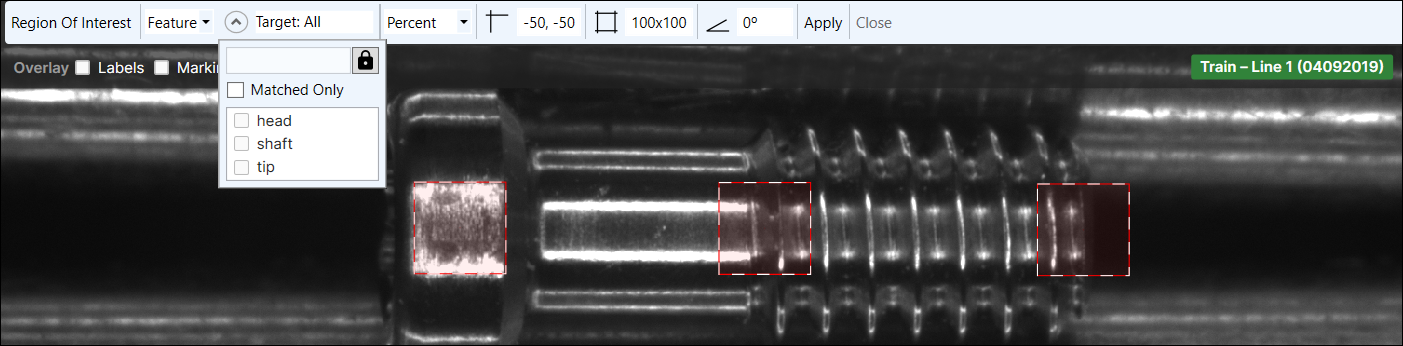 Note: By pressing the lock icon and disabling it, you can create your own expression for a feature or match filter of which features to use. You can construct custom filters around syntax using feature[] or match[], such as feature[id='featurename'] or match[name='modelname']. An empty filter (which is the default setting), will match all features.
 -
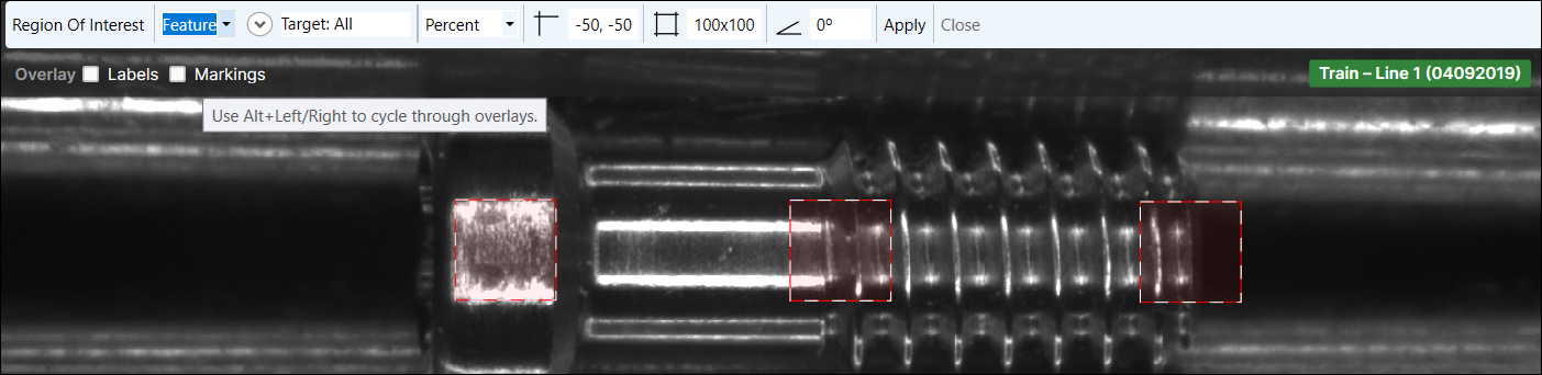
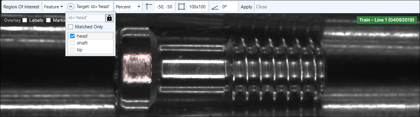
Select one or more features or Matched Only.
-
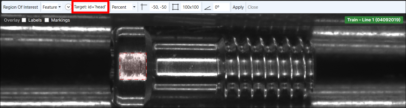
The Target field will display the filter being applied to generate views. You can then adjust the ROI to fit the area you want to inspect.
ROI from a Match
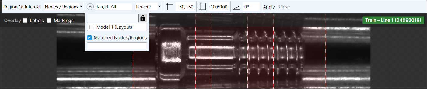
The Matched option allows you to specify that an ROI is only created if the preceding Blue Locate tool produces a matching node or layout model.
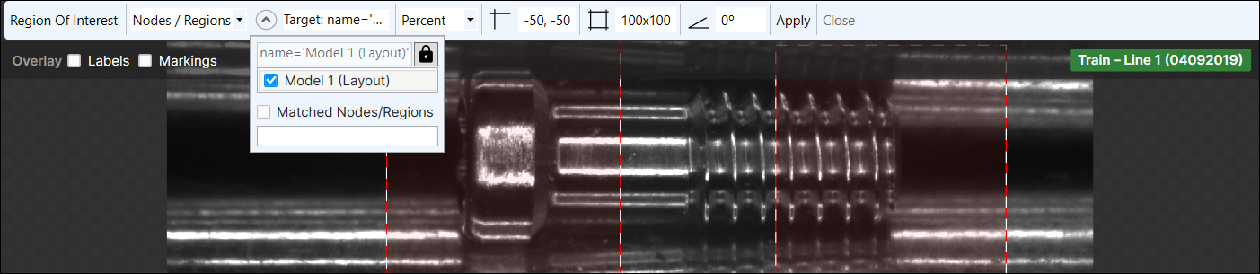
ROI from a Node or Layout Model
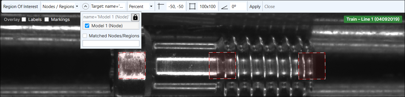
If a node model or a layout model has been configured, a tool following a Blue Locate tool can use a node or layout model to adjust the orientation of their region of interest (ROI).
A node model provides a five degree of freedom (DOF) transform (X translation, Y translation, rotation, X scale and Y scale). The node model will also determine the size of the ROI. The percentage of the ROI will be based on the width and height of the node model.
A layout model can also be used, which will present the various regions of the model as views for the downstream tool.
While in Expert Mode, the Scale setting is available, which scales the ROI to match the model reference frame. By default, the ROI does not scale, and uses the original image pixel size. In addition, you can also specify that only matches will be applied.
By pressing the lock icon and disabling it, you can create your own expression for a feature or match filter of which features to use. You can construct custom filters around syntax using feature[] or match[], such as feature[id='featurename'] or match[name='modelname']. An empty filter (which is the default setting), will match all features.
ROI Options Following a Green Classify Tool
When a Green Classify Tool is the preceding tool, a filter can be applied to only display views that match a specific tag for the following tool. The ROI for the tool after the Green tool can then be resized to fit the needs of your inspection.

For example, if you were wishing to further analyze an image based on the images that were classified as being of the tag '5', you could enter a couple of different expressions into the Filter field.
- best_tag='5' and score > threshold
- tag![5]/score > threshold
With these expressions as filters, only views that were tagged as '5' with a score above the Threshold parameter setting would be returned, since by the definition of the filter syntax, only views with a maximum score above the Threshold parameter are "found" by the Green Classify tool.
ROI Options Following a Red Analyze Tool
When a Red Analyze Tool is the preceding tool, there are several options for configuring the downstream tool.
-
You can manually configure the ROI by adjusting the ROI in the image. The default ROI toolbar is shown below. By not selecting any of the options in the toolbar, you can manually configure the size and location of the ROI to create the View.

- You can have the tool create individual ROIs for each defect that the preceding tool found.
-
You can have the tool not create an ROI if the preceding tool found a defect.

- You can apply a mask to the defect(s) in the ROI.
- You can reuse the mask from the preceding tool.
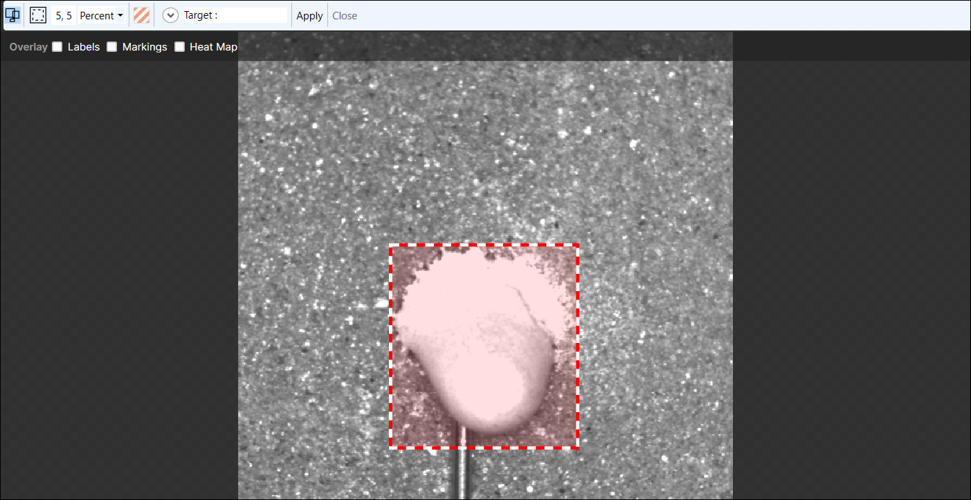
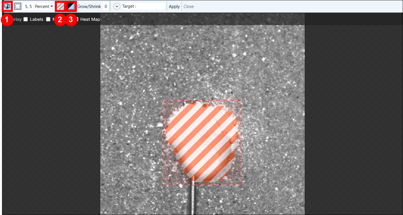
In the example below, the Extract regions as individual ROIs option is selected. With this option, found defects will be extracted from the image as individual regions, which will be converted into views.
You can also combine options, and add a mask inside the ROIs to exclude the background and only expose the defect.
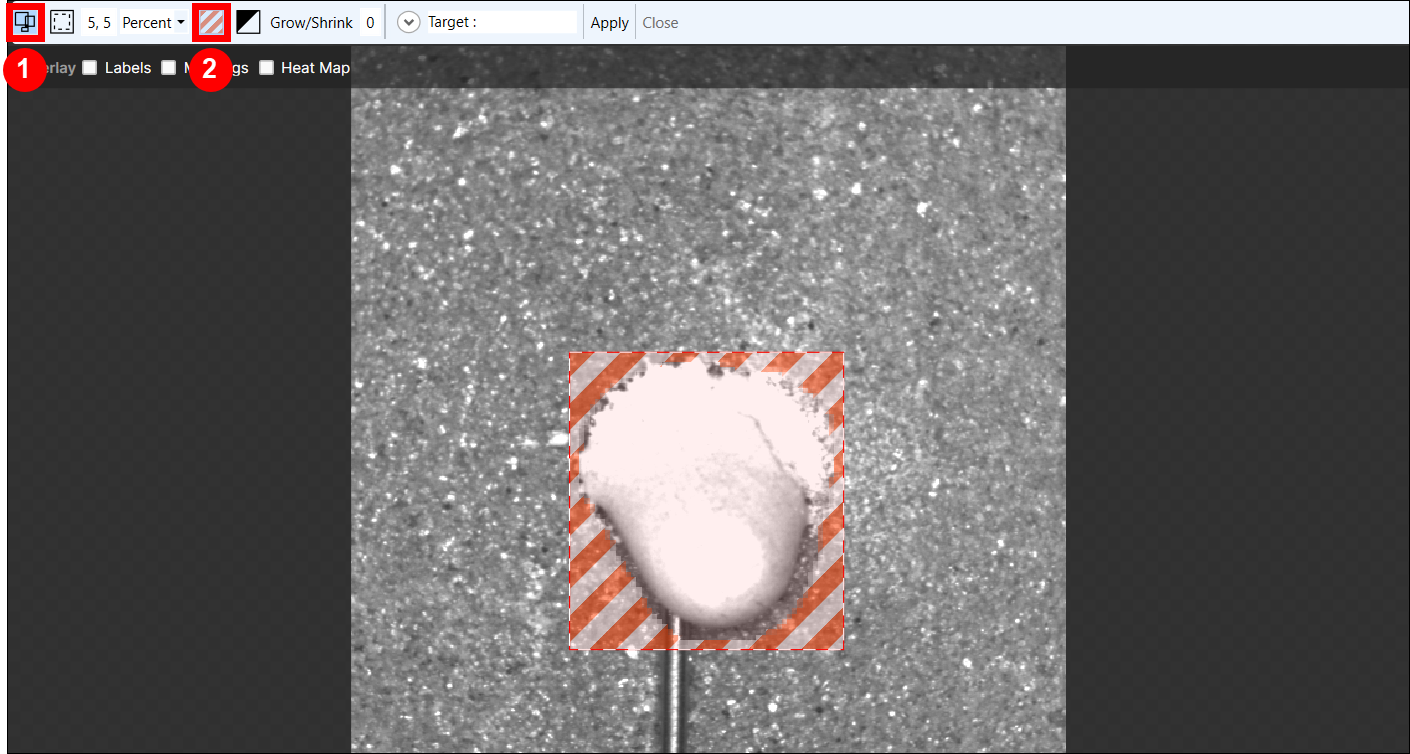
If you are more interested in the area outside of the defect, you can invert the mask to focus on the background instead of the defect.
Define a Mask for a Downstream Tool
When Cognex Deep Learning Tools are connected together in a tool chain, a mask that was created for a preceding tool will be used by the following tool(s). In this scenario, if a mask was created in Tool 1, and Tool 2 is chained to Tool 1, Tool 2 will inherit the mask of Tool 1. If you add an additional mask to Tool 2, while editing Tool 2, then Tool 2 will use both masks. To edit the mask of Tool 1 for use by Tool 2, you have to select Edit Mask while Tool 1 is the active tool.
Tool Chain Tutorial: Localize and Inspect Screws
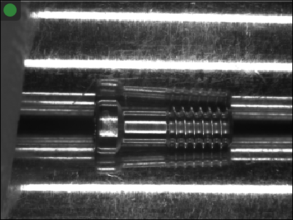
Screws or any other cylindrical object need to be rotated during inspection. Looking not only at one specific line along the rotation axis, but at the full object over several images, brings the advantage that you can see the surface and defects at different angles to the camera and the illumination. For instance, some defects will show best when they are on the center line, others will show better when they are slightly off to the sides.
Since the Red Analyze Tool does not rely on the precise positioning or orientation of the object, it can essentially operate in open loop. In other words, you can take a series of images (movie) of the rotating object and present them directly to the Red Analyze tool. In this particular set of images, however, the screws are moving across the entire image such that it is advisable to first use a Blue Locate Tool to localize and crop the screw before feeding it to the Red Analyze tool.
The objectives of this tutorial are:
-
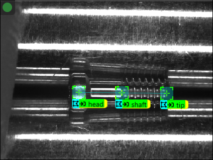
Use the Blue Locate tool to localize and track fuzzy features.
-
Generate a geometric model to find the screw's pose.
-
Configure a segmenter to process the screws by a Red Analyze tool.
-
Implement the Training Passes parameter to improve detection results.
- Add the images for the Screw tutorial.
- While in training mode, after a Workspace has been added or opened, images can be added through either the Database menu (select Add Images), by pressing Add Images in the display space of the GUI, or dragging and dropping images from a Windows Explorer directory into the View Browser.
- Add a Blue Locate tool.
- Adjust the ROI to segment an image, and then press the Scissors icon to process the images based on the new ROI.
- Set the Feature Size parameter to 80.
- Define at least two features (for example, the end and the tip of the screw) on at least three images.
- Press the Brain icon to train the system. Then review the results and manually label the images where the features were not found correctly.
- If you had to manually label new images, retrain the system and review the results.
- Right click on an image which has the two features and create a model named "screw".
- Reprocess the image and make sure the model is correctly found.
- Add a Red Analyze tool, and leave it in Unsupervised Mode.
- Segment the images for the Red Analyze tool by choosing the "screw" model.
- Change the size of the ROI to 700 x 250.
- Disable the Centered checkbox and use the mouse to move the ROI over the screw.
- Press Apply to segment all the images, and then verify that the images in the database are correctly segmented.
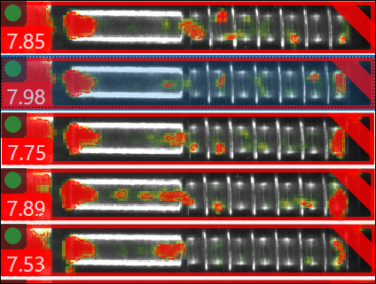
- Label all the images as good where the defect is not visible, and bad for the images where the defect is visible.
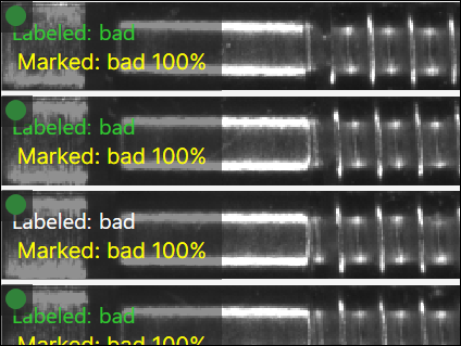
- Train the tool and verify the results.
- If the results are not satisfactory, increase the number of iterative trainings by increasing the Training Passes parameter and retrain.
Tool Chain Tutorial: Localize Orientation and Inspect Watch Dials
Watch dials and many other printed components demand high quality. Therefore, often pad printing (or tampography) is used, which, however, provides inspection challenges. If multiple pads are used, the alignment is often imperfect. The amount of ink applied changes such that the thickness of the lines may vary. While all this is not disturbing to the eye, it needs to be accepted. However, real defects like missing ink, spills or problems on the substrate need to be detected.
The images for this tutorial show watch dials at random orientations. You first need to use a Blue Locate Tool to determine the center and orientation of the dial. The resulting cropped and reoriented images can then be analyzed by a Red Analyze Tool. Since the dial also has holes which allow the presentation grid underneath it to be seen, you need to use a mask to prevent the Red Analyze tool from inspecting those areas.
The objectives of this tutorial are:
- Use the Blue Locate tool to localize and correct the orientation of the dial.
- Attach a Red Analyze tool to perform the inspection.
- Add a mask to control which areas are inspected and which are not.
- Add the images for the Dials tutorial.
- Add a Blue Locate tool.
- Segment the images by adjusting the ROI of the Blue Locate tool to enclose the watch dial.
- Set the Feature Size parameter to 100.
- Select at least two features (for example the center and the hole under the "B"), and label them in at least 3 images.
- Compensate for the variability in the orientation of the dial by adding some rotation during the training phase by changing the Rotation Perturbation parameter interval to [0,360].
- Train the system and review the results.
- Manually label any of the images where the features were not found correctly.
- If you had to manually label new images, retrain the system and review the results again.
- In one of the images, select two of the labeled features, right-click on the View and select Create Model from the menu and create a model named "dial".
- Reprocess the images and make sure the model is correctly found.
- Add a Red Analyze tool, and configure the ROI setting to use the "dial" model, and set the size of the ROI to 1850 x 1850.
- Segment all the images and verify that the images in the database are correctly segmented.
- Label all the images as Good, and then use the display filter to label the images which contain the word "bad" in their filename as Bad.
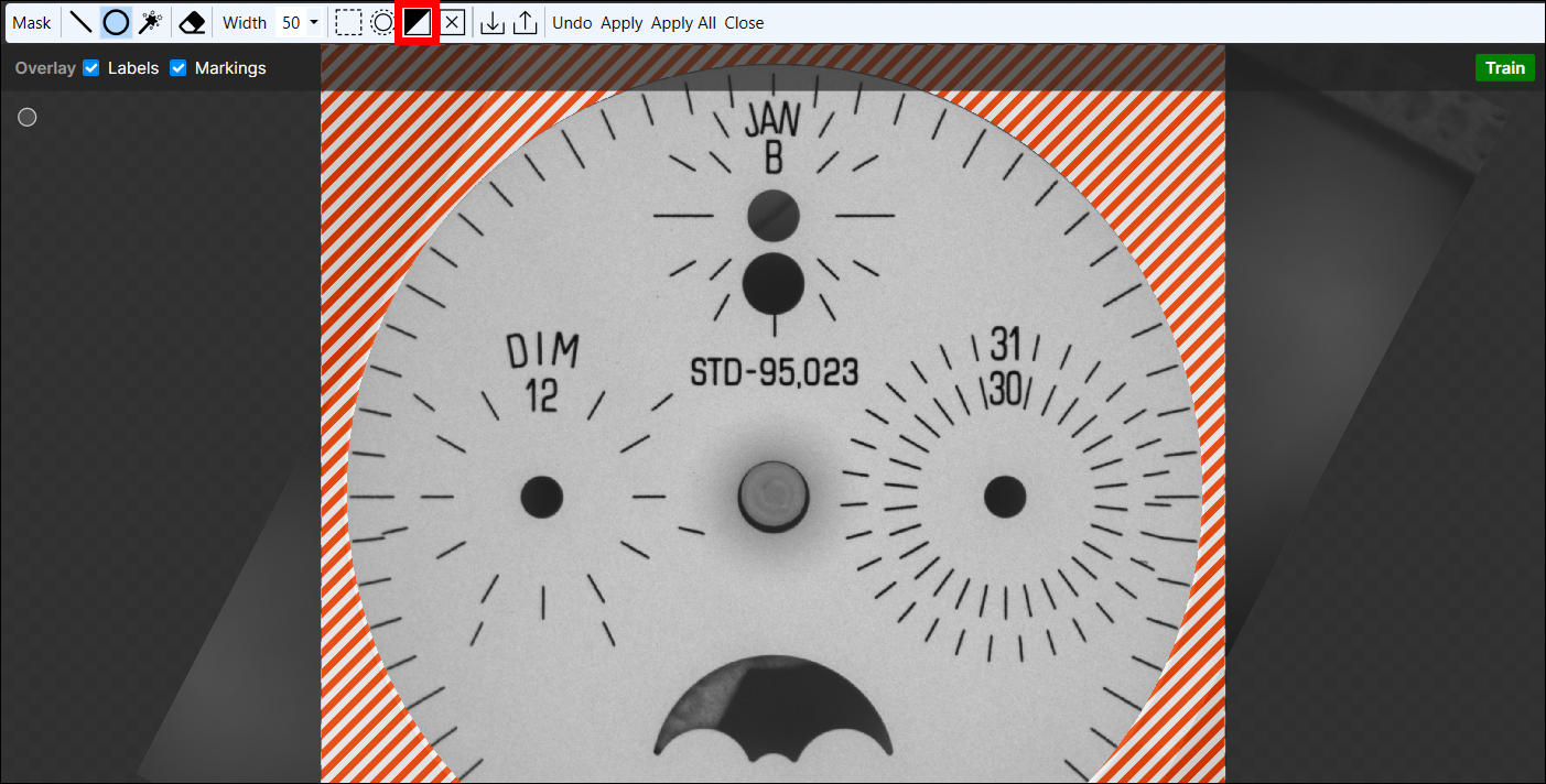
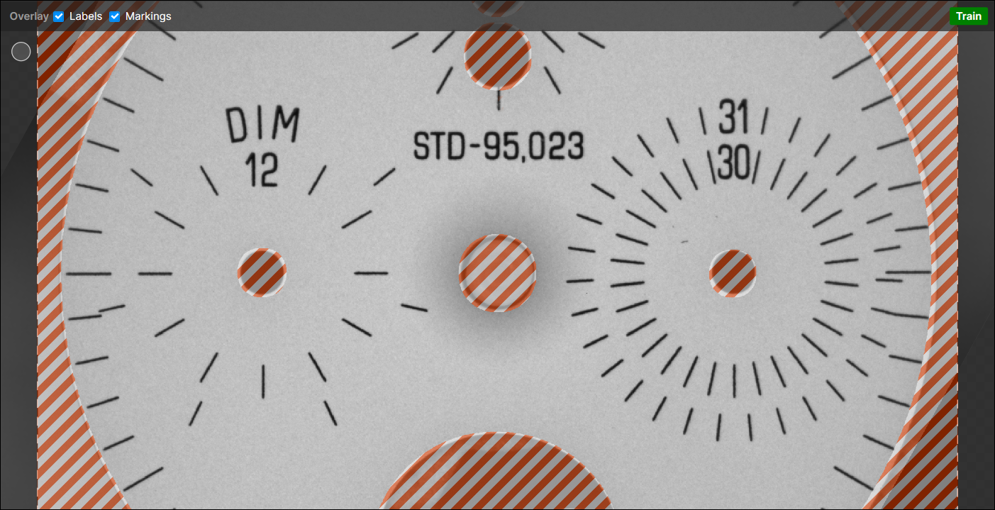
- Create a mask to hide the background, the small circles on the surface and the half-moon shape.
- In the Image Display Area, right-click and select Edit Mask from the menu.
Select the Circle Tool, and from the center of the dial, draw the circle outward to the edge.
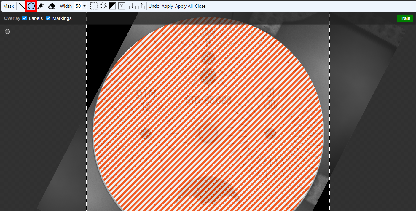
With the circle mask in place, press the Invert button to have the mask cover the outside of the circle.
Select the Circle Tool and apply circle masks to each of the other circular features in the image.
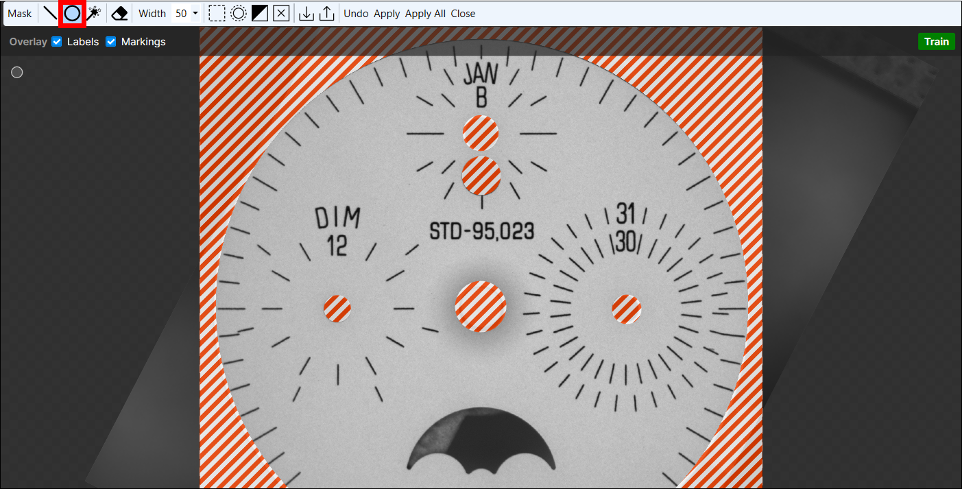
Select the Magic Wand tool, and holding down the Shift key, drag the wand over the shape to fill it in.
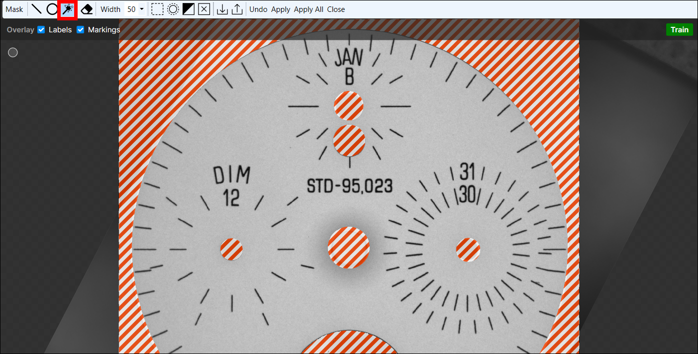
With all of the masks in place, press the Apply button, which will launch the Apply Mask dialog, allowing you to apply the mask to all of the images.
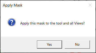
Press the Close button to close the Edit Mask phase. The mask should now be applied to all of the images.
- Train the tool and review the results, validating that the tool correctly marked the defects. If you have to adjust any of the parameters associated with training, or you have to re-label an image, you will need to retrain the tool and re-validate the results.